This article explains how to create some fractal plots with graphics.py, a popular graphics library for Python written by John Zelle. Graphics.py is a single file containing graphics functions such as Point, Line, Circle and Rectangle. Elsewhere on this blog, it’s been used to create sinusoidal patterns, including a Mexican hat/blancmange surface. This article focuses on the creation of fractal images.

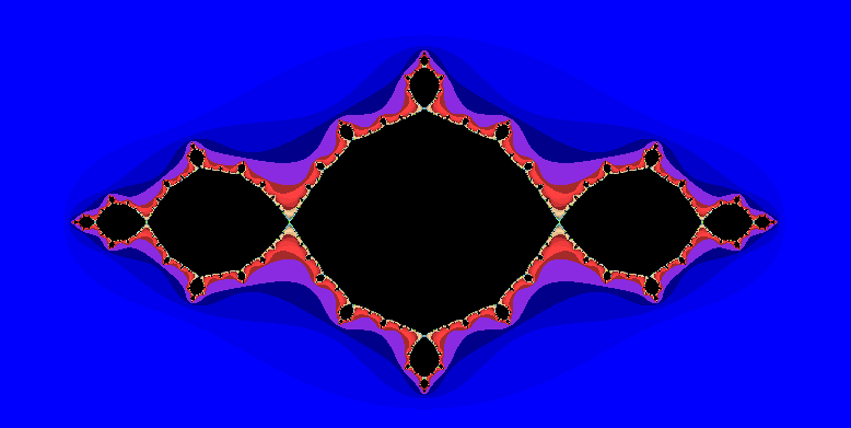
Install Graphics.py

Install graphics.py as follows:

pip install graphics.py

Install Julia.py

julia.py is a small program for plotting Julia and Mandelbrot sets. It’s just a quick learning aid for gaining appreciation of these sets and the simple algorithms that produce them. Grab julia.py now, and set its permissions:

$ curl -O https://raw.githubusercontent.com/webtaster/Julia/master/julia.py
$ chmod 755 julia.py

…and the tkColors.py library, which needs to stay in your current working directory.

$ curl -O https://raw.githubusercontent.com/webtaster/Julia/master/tkColors.py

Plot a Julia Set

Run the program. A graphics window should appear, and a classic Julia set will be drawn, just like the one pictured above. Be patient. The plotting can take 30 seconds or more. That’s how long it took on my powerful but ageing laptop (containing a 4th generation Intel i7 CPU).

What you are looking at (hopefully) is a classic Julia set, similar to Plot 1 (above) and to this example at Michael Goodwin’s site. Meanwhile, some information appears in the shell:

$ ./julia.py
Type: Julia, c = (-1+0j)
zoom factor 200
most iterations 40
Done

Click the mouse for information on a point, or ctrl-c to end

Press ctrl-c in the shell to exit the program.

Varying the Constant

A Julia set can be varied by changing the c constant. Do so now. Edit julia.py and change line 119 so that the new value of c becomes:

c = complex(-0.512511498387847167, 0.521295573094847167)

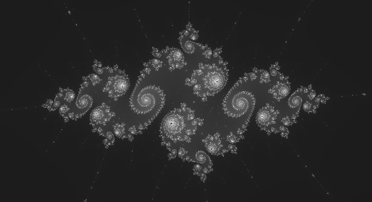
These c values are taken from the first example on the Wikipedia Julia Set page, and the image produced (below) closely resembles the Wikipedia rendering. But not before we make one more edit. Comment line 58 and uncomment line 63, changing the output from multi-colour to graduated monochrome:

  # Colourful, a bit random but clear
  #color = tkColors[(a+25) % 750]

  # Uncomment for a nice graded monochome rendering.  Increases plot time.
  color = color_rgb(a*4, a*4, a*4)

Now run it, and you should see:

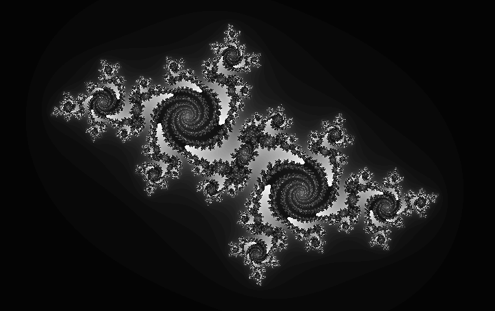
Slightly changing the value of c has resulted in a big change in the output image. Switching from colour rendering to monochrome makes the details, and the resemblance to Wikipedia’s version, easier to see.

Undo your edits to julia.py before proceeding. Or just download it again:

curl -O https://raw.githubusercontent.com/webtaster/Julia/master/julia.py

Mandlebrot Sets

The Mandelbrot set is like the Julia set, except that the value of c isn’t constant. It varies with each point on the plane, taking the complex value of that point. Simple to program, because the Julia/Mandelbrot code needs differ by just a few characters, (viz. line 217: ‘c = z’).

Also, there is just 1 Mandelbrot set, whereas there are many Julia sets – we plotted 2 of them above. Anyway, draw the Mandelbrot set now. Edit julia.py. Change line 114 from

julia = True

to

julia = False

and run the program:

./julia.py

Up comes the familiar Mandelbrot shape, complete with garish colourisation:

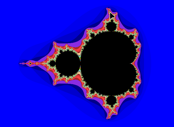
When the Mandelbrot set has finished drawing, click your mouse in the graphics window, just where you see the pointer/cursor in the above image. A set of coordinates will be printed to the terminal, something like:

x_offset = -0.15265265265265243
y_offset = 1.0287859824780976

These numbers will come in useful presently.

Mandelbrot Zoom In

Being a fractal, the Mandelbrot plot responds well to zooming in, the effect of which is to reveal ever more detail. Edit julia.py again, go to lines 103 to 104, and insert the x_offset and y_offset values, just as they are written above. Next, edit line 98 and change the value of the ‘zoom‘ variable to 5000. This will increase the existing zoom in by a factor of 25. Save julia.py.

Run the program:

$ ./julia.py

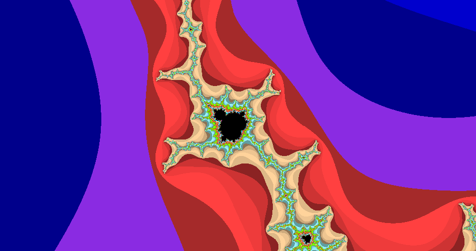
What has been revealed here is a common feature of the set, known for obvious reasons as a “mini Mandelbrot”. The area in the middle of this image has a shape similar to the overall set.

Mandelbrot Browsing with julia.py

If you like, it is possible to explore the Mandelbrot set by repeatedly applying this zoom and offset technique. Draw an image, click the mouse on an interesting looking place, put the printed coordinates back into julia.py, increase the zoom, and re-run. And repeat. Interesting features or especially decorative areas can be plotted. For example, there are many mini Mandelbrots, including some at levels of zoom much higher than that shown in Plot 4.

Professional Browsers

For serious exploration, there are also many excellent Mandelbrot browsers online. These are professional quality, with real time zoom and pan. For example, here’s how mandel.gart.nz interprets the same area from Plot 4:

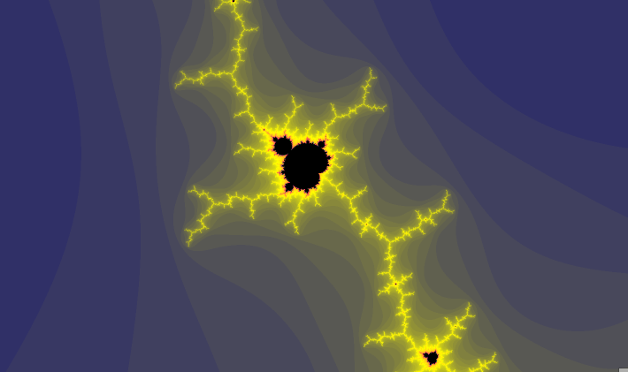
Try the “I Feel Lucky” button over at bertbaron.github.io. Also easy on the eye, with a calm default colour scheme, is mandelbrot.site.

Well Known Features

An intriguing feature of mandel.gart.nz is the invitation to “Jump to” a list of well known Mandelbrot beauty spots, including “Seahorse Valley”, “Julia Island” and “Star Fish”. Some of these are at mind-blowing magnifications. For example, select Julia Island, and enjoy an animated journey down to zoom level 1,585,714,676, where this comely figure lives:

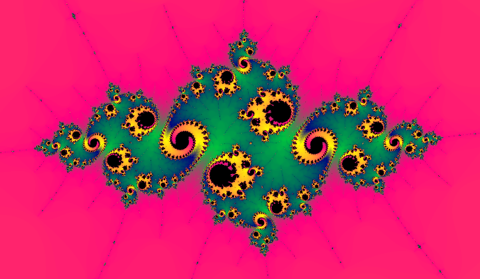
Julia Island

Here’s how our humble julia.py draws Julia Island. Edit the program as before, changing the offsets and zoom again, as follows, then run it. NB. the coordinates came straight from mandel.gart.nz.

zoom = 792857338

x_offset = -1.768778833
y_offset = -0.001738996

./julia.py

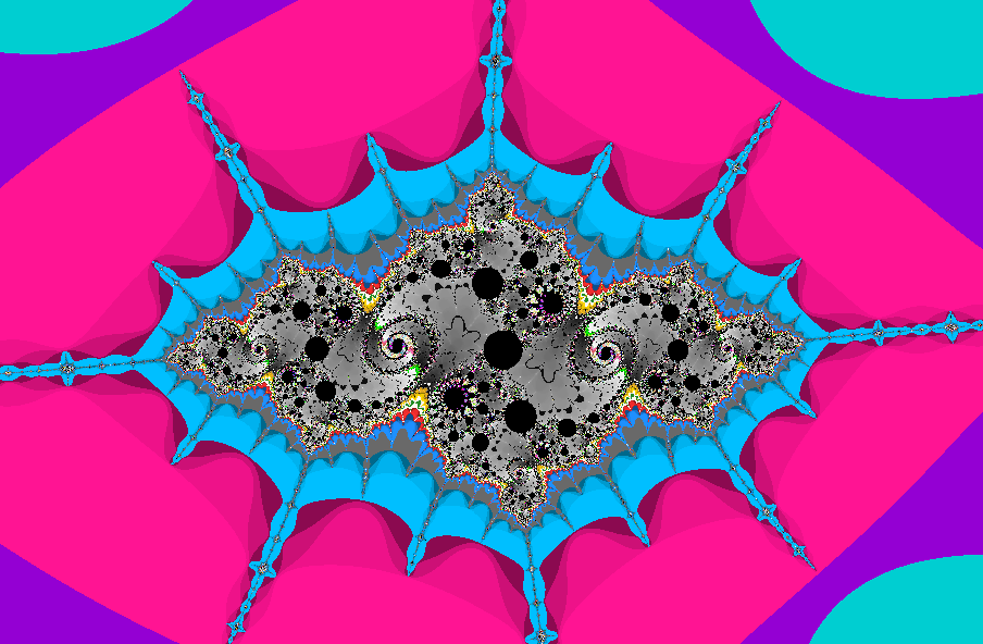
There are some differences this image (Plot 7) and the one produced by mandel.gart.nz (plot 6). Apart from the colour scheme, our home-made plot has a central “hole”, a black disk, which does not appear in mandel or other online renderings. Plot 8 shows the effect of increasing maxitr, (line 149), one of the rarely adjusted settings, to 2000, and swapping to monochrome:

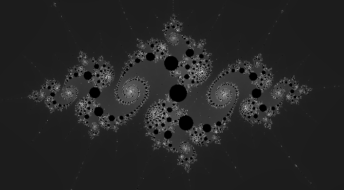
Plot 8 is better, but we still have those holes. Decreasing the zero_threshold from 0.01 to 0.00001 (line 146) improves matters, as shown in plot 9:

Shrinking the zero_threshold reduced the level at which the algorithm deems a complex value to have imploded to near zero. Areas that were previously black, like those unexpected black disks in Plot 7, must have had a value (an absolute size) between 0.01 and 0.00001. Now the algorithm considers them non-zero, instead of zero, and they are colourised accordingly.

Changing the Complex Function

It is possible to change the complex series itself, resulting in further fractal sets. For a quick example, “reset” julia.py by downloading it again.

curl -O https://raw.githubusercontent.com/webtaster/Julia/master/julia.py

Now we are back to plotting Julia sets. Running the program now would yield the same image as in Plot 1, above. Go to line 31. This is the main complex equation and the heart of the program. Change it from

z = z*z + c

to

z = z*z*z + c

or even

z = z*z*z*z*z + c

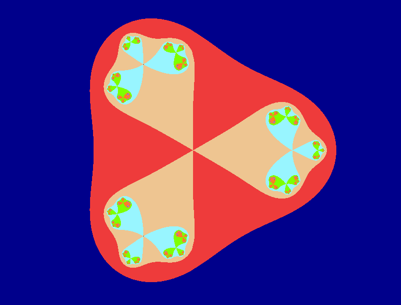
Run the program to display the higher order Julia set. These can also be zoomed-in on, of course, showing the effect of the polynomial. Z cubed functions tend to produce images with a 3 lobe motif. Z to the power of 5 five tends to make quintuple visual effects. The plot below is a julia set, with the function modified to z = z*z*z + c.

Conclusion

This article could go on longer, citing more and more Fractal examples. With Mandelbrot and Julia sets being fractal, there is an infinite amount of detail to explore. I hope it has been an interesting read and not too waffly.

There are many online resources for visualising Julia and Mandelbrot sets. Apart from sites mentioned in the above section entitled “Professional Browsers” there excellent pages and especially YouTube videos explaining with detail and clarity the underlying mathematics.

For an everyday illustration, this effort on the Numberphile channel, “What’s so Special about the Mandelbrot Set?“, is hard to beat.

Another kind of satisfaction can be obtained by drawing these things in a do-it-yourself manner, with a simple program like julia.py, or similar, making alterations and seeing their affect on the output. The simplicity behind the Mandelbrot and Julia sets forms a large part of their fascination.

Appendix

Improvements to Julia.py

julia.py is just a quick program, designed to aid understanding the Mandelbrot algorithm. As such, it has been left plain and unoptimised. From a programming point of view, there is much scope for improvement. Eg. tidying the code into proper functions, making it more readable, adding command line arguments to replace tiresome editing, making it multi threaded, optimising the iteration loop, and so on.

Computing Notes

Even on a multi core machine, julia.py is quite slow, because it is single threaded. On my 8 core laptop, one core is busy, while the others are relatively idle.

Building the image also takes a surprising amount of memory. As the Julia set in Plot 1 is drawn, memory consumption increases steadily, eventually reaching 495 MB as the image completes. This can’t be explained simply by the image size, which by default is 1000*800 pixels, implying 648 bytes per pixel. Plainly, the structures behind Graphics.py are sizeable.

A Note on Zoom Factors

For some reason, to produce an image of comparable size, the zoom factor within julia.py has to be about half that of the online fractal browsers. Not a big problem. It means julia.py’s images are about twice as big as those found online. Perhaps due to differences in screen size.

END.