
This article explains how to create some simple mathematical shapes with graphics.py, a popular graphics library for Python written by John Zelle. Graphics.py is a single file containing graphics functions such as Point, Line, Circle and Rectangle. In this article though, we are just going to use it to plot single points.
At the top of the page is a blancmange like shape. The program that drew it is at the bottom of the article, if you want to jump straight there. Otherwise, a couple of simpler plots will be demonstrated first, just to show a couple of underlying principles.
Install Graphics.py
Installing graphics.py can be as simple as downloading the latest version of the file. You can just leave it in the same directory as your python script.
$ wget https://mcsp.wartburg.edu/zelle/python/graphics.py
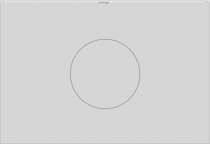
Plot a Circle
With graphics.py installed, run the following Python script. It will draw a circle by plotting sine against cosine:
#!/usr/bin/python

from __future__ import division
from graphics import *
import math

height  = 800
width   = 1200
radius  = 200

win = GraphWin(sys.argv[0], width, height, autoflush=False)
win.setCoords(-width/2, -height/2, width/2, height/2)

for a in range(0,360):

   ar = math.radians(a)

   pt = Point(radius*math.sin(ar), radius*math.cos(ar))   # Circle
   #pt = Point(2*radius*math.sin(ar), radius*math.cos(ar))  # Elipse
   #pt = Point(radius*math.sin(2*ar), radius*math.cos(3*ar))  # Lissajous

   pt.draw(win)
   win.update()

print "Done"

win.getMouse() # Pause to view result
win.close()
Run the program and a window should appear, looking like the image below. When you are ready, click the window to dismiss it and end the program.
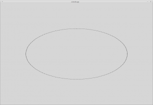
Plot an Ellipse
Edit the above script. Change the “pt = ” line to add a multiplying factor of “2*” to the x coordinate. Or, just uncomment the “Ellipse” line and comment out the “Circle” line.
Run the program and it now draws am ellipse. Basically just a squashed circle, twice as wide as it is high:
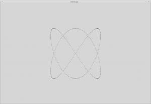
Lissajous Figure
If you introduce a multiplying factor to the angle (a) instead, a different effect is seen. Edit the program. Comment out the “Elipse” line and uncomment the “Lissajous” line. This is like the circle again, except that the x angle is multiplied by 2 and the y angle by 3.
Run the program and a swoopy pattern appears. It is still a plot of sine against cosine, but the “frequencies”, or wavelengths, of x and y are out by a factor of 1.5. You can vary those numbers to produce more complicated patterns.
Blancmange
At the top of this article is a figure shaped a bit like a blancmange, or a sort of Mexican hat. The program to draw it is below. It can also be downloaded directly from Github, or with wget, like so:
$ wget https://raw.githubusercontent.com/webtaster/Blancmange/master/blanc.py
More accurately, the shape could be called a radial sinusoid, decaying as 1/x from the origin. Although it might seem more complicated than the plots above, this “3D” surface plot is built using similar principles. Plot sine against cosine and you get a circle (a trigonometrical identity). Plot sin or cos alone and you get a wave. Pythagoras can be used to work out radial distances.
#!/usr/bin/python

from __future__ import division
from graphics import *
import math

# Dimensions of graphics window
height  = 800
width   = 1200

# Radius of shape about the Y axis
radius      = 400

# Viewing angle, in degrees to the horizontal
va          = 10

# Wavelength of sine wave in pixels
wavelength  = 170

# Height of the figure at the centre (see exponential decay, below)
centre_amplitude = 500

# Plot granularity.  Affects texture but not overall shape
xstep = 1
zstep = 10

# Viewing angle doesn't change, so calculate its sine and cosine now (optimization).
var     = math.radians(va)
sinvar  = math.sin(var)
cosvar  = math.cos(var)

win = GraphWin(sys.argv[0], width, height, autoflush=False)
win.setCoords(-width/2, -height/2, width/2, height/2)


# Image is symmetrical, so iterate x over half the  full range (-radius to radius)
# and plot both halves at the same time (optimisation).
for x in range(-radius, 0, xstep):

   # Pre-set maximums for hidden surface removal later
   maxy = -height
   miny = height

   # Optimisation: calculate and store this once instead of for every z later
   xsquared = x*x

   # The start (and end) of the z range for this x.  Pythagoras.
   zlimit = int(math.sqrt(radius*radius - xsquared))


   # This range is really just -zlimit to zlimit, step zstep.  The reverse
   # and addition here is just so that the range is symmetrical about zero,
   # making the pixels line up properly even at high viewing angles.
   # A simply range(-zlimit, zlimit) produces the same shape but the
   # texture is not uniform.
   for z in list(reversed(range(0, -zlimit, -zstep))) + range(0, zlimit, zstep):

      # Distance of this point from the Y axis, horizontally.
      r   = math.sqrt(xsquared + z*z)


      # Amplitude of wave
      # Reciprocal decay: more pointy
      amplitude = 5000*(1/(0.5*r+1))
      # Exponential decay: smoother
      #amplitude = centre_amplitude*(0.990**r)

      # y is a sinusoid of r, giving the wavy shape.
      y  = amplitude*math.sin(math.radians(r*(360/wavelength)))

      # "Rotate" the 3D image towards the viewer, about the x axis, to give
      # the viewing angle projection
      projy = z*sinvar + y*cosvar


      # Plot the points
      if (projy > maxy) or (projy < miny):
         pt  = Point(x, projy)
         pt.draw(win)
         pt  = Point(-x, projy)
         pt.draw(win)

      # Hidden surface removal
      if projy > maxy:
         maxy = projy

      if projy < miny:
         miny = projy

   # Tp speed up the drawing, remove the indent of the following line
   # To slow down, increase the indent, putting it into the z loop
   win.update()

# Wait for user to click on image or terminate program
print "Done"
win.getMouse()
win.close()
The shape takes about half a second to draw on my i7 laptop, and about 8 seconds on a raspberry pi 2. For comparison, I plotted the same curve using BASIC on an Amstrad CPC464 in the late 1980’s, where it finished in about 5 minutes (and that was with a radius of about 200, not 400). On a Dragon 32 (8 bit, 0.6 Mhz) took about 10 minutes or more.
Change the Parameters
Altering some parameters near the top of the script changes the produced image. For example, try changing the viewing angle, va (currently 10 degrees) to different values between 0 and 90. It represents the angle above the horizontal from which the user sees the image. The effect of radius is fairly obvious. Reducing the wavelength will give you more ripples.
Changing the “decay” rate alters the steepness of the shape. Fiddle with the main “y=” statement, and you can draw different shapes altogether.
Notes
Inserting the blancmange routine into a function and calling it with increasing va (viewing angle), and blanking the screen appropriately, produces a nice animation. It is only practical on a quick machine though, and will be far too slow on a Raspberry Pi.
Acknowledgements
I originally got the “blancmange” algorithm from a 1980s UK computer magazine. But I can’t recall which one it was, let alone the name of the author. Thanks anyway!
Update – I think it might have been UK computer magazine Your Computer, November 1982. Page 22, “Opening Up Graphics“. If so, thanks to Mr Tim Langdon! All done in 10 lines too – program D4.
That image at the top took me back! Before reading further it was reminding me of graphics I played with on a Tandy CoCo in early-mid 1980s, some preserved by me taking photos of the TV screen as they were displayed. Same hardware as the Dragon 32 but mine had an awesome upgrade to 64k of memory
Hi Adrian, that is very cool! Sorry about the delay in replying, just been on an Easter break. Yes, the CoCo and Dragon were essentially the same computer. Back in the 80s, I printed out the image at the top, but the printouts have long been lost. If you want to send a photo, or part of a photo, I will add it here.
64k – awesome
Pingback: Simple Julia and Mandlebrot Sets with Python | Unix etc.